From TRPO to PPO
The fundamental problem of policy optimization
In supervised learning, updating parameters doesn’t change the data. In RL, updating the policy changes which states you visit, which changes the data distribution. The optimization landscape shifts under your feet with every gradient step.
This is why vanilla policy gradient is unstable. A step that looks good under the current data distribution might be catastrophic once the visitation frequencies change.
The surrogate is a tangent plane
Consider policy improvement. The true objective under $\tilde{\pi}$ :
\[\eta(\tilde{\pi}) = \eta(\pi) + \sum_{s} \rho^{\textcolor{red}{\tilde{\pi}}}(s) \sum_{a} \tilde{\pi}(a \mid s) A^{\pi}(s, a)\]The surrogate :
\[L_{\pi}(\tilde{\pi}) = \eta(\pi) + \sum_{s} \rho^{\textcolor{red}{\pi}}(s) \sum_{a} \tilde{\pi}(a \mid s) A^{\pi}(s, a)\]The only difference : $\rho^{\tilde{\pi}}$ vs $\rho^{\pi}$. The surrogate pretends the state distribution doesn’t change. This is the fundamental lie of policy gradient.
$L$ is a first-order approximation — a tangent plane to $\eta$ at $\pi$. Near $\pi$, the tangent plane is accurate. Far from $\pi$, it diverges from reality. The question is : how far can you go before the lie breaks?
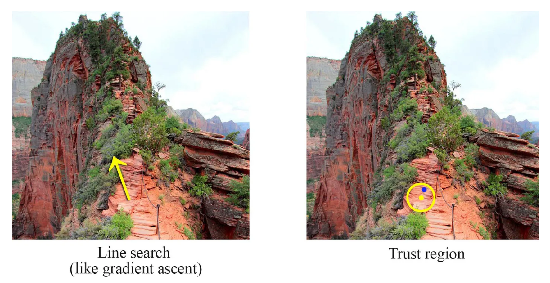
The trust region
Kakade and Langford (2002) gave the answer :
\[\eta(\tilde{\pi}) \geq L_{\pi}(\tilde{\pi}) - C \cdot D_{KL}^{\max}(\pi \| \tilde{\pi})\]The KL divergence bounds how much the visitation frequencies can diverge. In the theoretical exact update with the worst-case KL bound, stay within the trust region and monotonic improvement is guaranteed. Practical TRPO only approximates this.
\[D_{TV}^2 \leq \frac{1}{2} D_{KL}\]TRPO : natural gradient on policy space
\[\max_\pi \; \mathbb{E}\_{s \sim \rho^{\pi_{old}}, a \sim \pi_{old}} \left[ \frac{\pi(a|s)}{\pi_{old}(a|s)} A^{\pi_{old}}(s,a) \right] \quad \text{s.t.} \quad D_{KL}(\pi_{old} \| \pi) \leq \delta\]The step direction is approximately $F^{-1}g$ — the natural gradient. The Fisher information matrix $F$ defines the Riemannian metric on policy space. It measures how much the distribution changes, not how much the parameters change.
A large parameter change that barely affects the output distribution is “small” in this metric. A tiny parameter change that flips the policy is “large.” This is the right geometry for optimization over distributions.
Solved via conjugate gradient + line search. Elegant, but expensive — the Fisher-vector products are the bottleneck.
PPO : when theory meets practice
Schulman’s key observation : TRPO’s monotonic improvement guarantee requires exact optimization of the surrogate. In practice, you do approximate SGD with finite samples and mini-batches. The theoretical guarantee is already broken by implementation.
If the theory is already approximate, use whatever works.
\[L^{CLIP}(\theta) = \mathbb{E} \left[ \min \left( r_t(\theta) A_t, \; \text{clip}(r_t(\theta), 1-\epsilon, 1+\epsilon) A_t \right) \right]\]The clipping discourages catastrophic updates — but the ratio itself can still go too far. Clipping flattens the surrogate contribution outside the interval; it is not a hard trust-region constraint. No second-order optimization. No conjugate gradient. No line search. First-order SGD, runs on any framework, parallelizes trivially.
PPO doesn’t have TRPO’s theoretical guarantees. It doesn’t need them to be useful — those guarantees were already approximated in practical TRPO. What it has is a cheap mechanism that usually prevents the policy from jumping off a cliff, though not a hard guarantee that it cannot.
Many people use PPO without understanding it. But that’s exactly why it’s a good algorithm.
References